
Distributions
Bar Chart vs Histogram: Differences & Examples
A category bar chart compares named groups. A histogram groups measurements into numeric intervals to show their distribution. Both may show counts, but they answer different questions. ChartPetal supports category bars; the histogram illustrations here are educational and do not imply an automatic histogram feature.
Category bars: deliveries by carrier
Educational histogram: five-minute bins
In this guide
Two questions for the same twenty deliveries
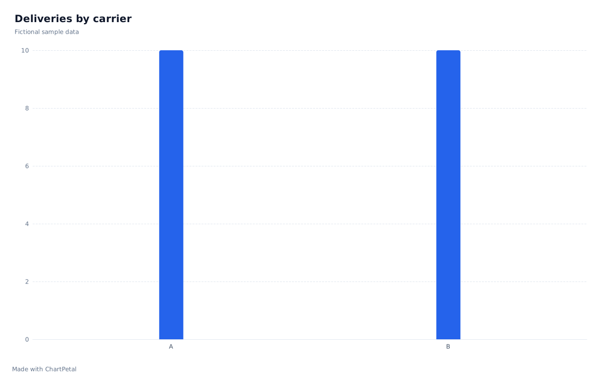
The fictional source table pairs a carrier with a duration in minutes for each delivery. Counting rows by Carrier gives ten for A and ten for B: it answers how many deliveries each handled. A histogram uses DeliveryMinutes instead, pooling both carriers to ask where durations are concentrated. The equal carrier counts tell you nothing about equal delivery speed.
| Carrier | DeliveryMinutes |
|---|---|
| A | 2 |
| A | 4 |
| A | 5 |
| A | 7 |
| A | 8 |
| A | 9 |
| A | 11 |
| A | 12 |
| A | 14 |
| A | 18 |
| B | 3 |
| B | 6 |
| B | 6 |
| B | 8 |
| B | 10 |
| B | 13 |
| B | 15 |
| B | 16 |
| B | 17 |
| B | 19 |
Define the bins before counting
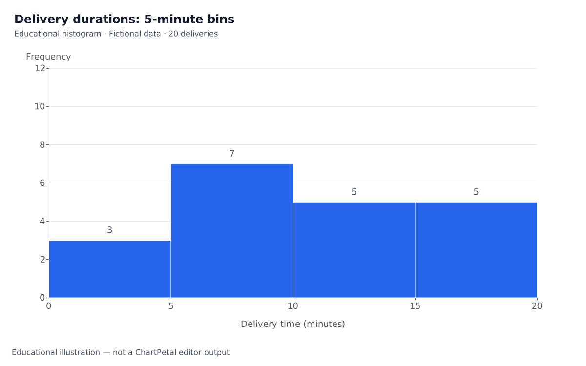
For this sample, each interval includes its lower bound and excludes its upper bound: 0 ≤ minutes < 5, 5 ≤ minutes < 10, 10 ≤ minutes < 15 and 15 ≤ minutes < 20. The counts are 3, 7, 5 and 5, totaling 20. A value of 5 goes into the second bin, and 10 into the third. Every source value is at least 0 and below 20; a future value of 20 would need an additional interval or an explicitly revised final boundary.
Bin width changes the visible shape
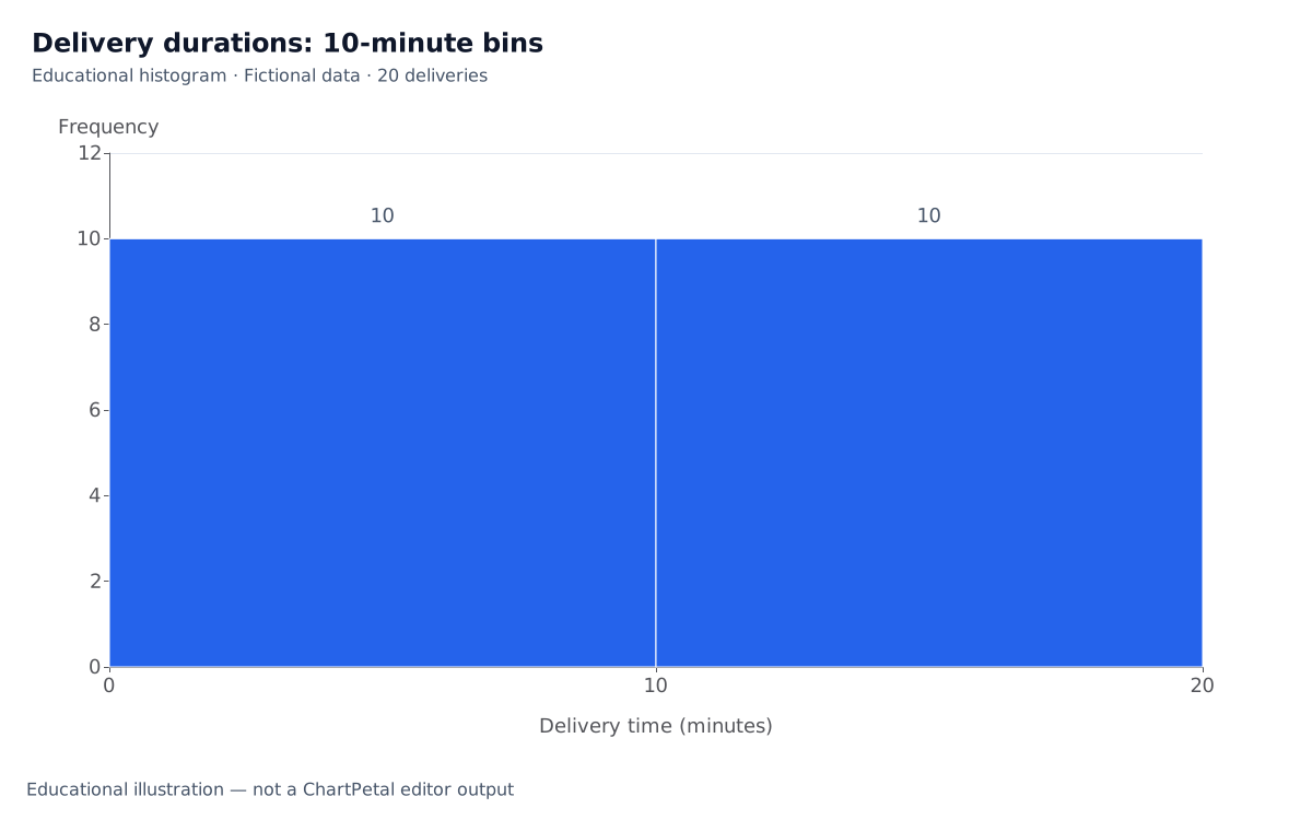
Combining each adjacent pair into ten-minute intervals gives counts of 10 and 10. The measurements have not changed, but the broader grouping hides the difference between the first two five-minute intervals. Try plausible widths and report the boundaries. With only twenty fictional observations, do not infer a population distribution or service guarantee from the apparent shape.
The educational histograms use a numeric horizontal scale, adjacent intervals and equal widths within each chart. Category bars use separate labels and can be reordered for a different comparison. A numeric distribution must retain interval order. For unequal-width histogram bins, raw count heights are misleading: density must account for bin width so area represents frequency. The equal-width example here avoids that extra calculation.
Educational histogram: ten-minute bins
What you can reproduce in ChartPetal today
Use Edit the category count chart to open the raw table with Bar, Carrier as X and Count as Aggregation. For a frequency summary, download the provided Bin and Frequency table and open Edit the pre-binned frequency bars. It selects Bar, Bin as X, Frequency as Values and None as Aggregation, preserving the four interval labels in input order. Count would count table rows instead of using the frequencies 3, 7, 5 and 5.
The pre-binned result is a categorical frequency bar chart with separated bars. It is not a continuous-axis histogram. ChartPetal does not choose bin boundaries, bin raw numeric measurements, control histogram bin width or compute density. Changing the raw table does not recalculate the supplied frequency table. Recalculate bins in your spreadsheet or a statistical tool, then import the new frequency values.
| Bin | Frequency |
|---|---|
| 0 <= minutes < 5 | 3 |
| 5 <= minutes < 10 | 7 |
| 10 <= minutes < 15 | 5 |
| 15 <= minutes < 20 | 5 |